


Cache-Friendly, Low-Memory Lanczos Algorithm in Rust

Cache-Friendly, Low-Memory Lanczos Algorithm in Rust
The standard Lanczos method for computing matrix functions has a brutal memory requirement: storing an
In this post, we will explore one of the most straightforward solutions to this problem: a two-pass variant of the Lanczos algorithm that only requires
- All code is available on GitHub: two-pass-lanczos
- The full technical report with proofs and additional experiments: report.pdf
Table of Contents
Open Table of Contents
Computing Matrix Functions
Let’s consider the problem of computing the action of matrix functions on a vector:
where
Indeed, there are a lot problems with computing
However we know that given any matrix function
This gives us a good and a bad news: the good news is that, well, we can express
This polynomial only involves vectors within a specific subspace.
Krylov Projection
We can notice that
This is fortunate: we can compute an approximate solution by staying within this space, which only requires repeated matrix-vector products with
We don’t need to construct
A j \mathbf{A}^j Aj explicitly. We compute iteratively:A ( A j − 1 b ) \mathbf{A}(\mathbf{A}^{j-1}\mathbf{b}) A(Aj−1b).
But there’s a problem: the raw vectors
Building an Orthonormal Basis
The standard method is the Arnoldi process, which is Gram-Schmidt applied to Krylov subspaces. We start by normalizing
- Compute a new candidate:
w j = A v j \mathbf{w}_j = \mathbf{A}\mathbf{v}_j wj=Avj - Orthogonalize against all existing basis vectors:
- Normalize:
v j + 1 = v ~ j / ∥ v ~ j ∥ 2 \mathbf{v}_{j+1} = \tilde{\mathbf{v}}_j / \|\tilde{\mathbf{v}}_j\|_2 vj+1=v~j/∥v~j∥2
The coefficients
V k = [ v 1 , … , v k ] \mathbf{V}_k = [\mathbf{v}_1, \ldots, \mathbf{v}_k] Vk=[v1,…,vk]: an orthonormal basis forK k ( A , b ) \mathcal{K}_k(\mathbf{A}, \mathbf{b}) Kk(A,b)H k \mathbf{H}_k Hk: an upper Hessenberg matrix representing the projection ofA \mathbf{A} A onto this subspace
We can express this relationship with the Arnoldi decomposition:
Solving in the Reduced Space
Now we approximate our original problem by solving it in the small
where
The heavy lifting is now on computing
For
f ( z ) = z − 1 f(z) = z^{-1} f(z)=z−1 (linear systems), this reduces to solvingH k y k = e 1 ∥ b ∥ 2 \mathbf{H}_k \mathbf{y}_k = \mathbf{e}_1 \|\mathbf{b}\|_2 Hkyk=e1∥b∥2 with LU decomposition.
The Lanczos Algorithm
When
In the literature, this projected matrix is denoted
where
Three-Term Recurrence
This tridiagonal structure leads to a beautiful simplification. To build the next basis
vector
Rearranging gives us an algorithm to compute
- Compute the candidate:
w j + 1 = A v j w_{j+1} = \mathbf{A}\mathbf{v}_j wj+1=Avj - Extract the diagonal coefficient:
α j = v j H w j + 1 \alpha_j = \mathbf{v}_j^H w_{j+1} αj=vjHwj+1 - Orthogonalize against the two previous vectors:
- Normalize:
β j = ∥ v ~ j + 1 ∥ 2 \beta_j = \|\tilde{\mathbf{v}}_{j+1}\|_2 βj=∥v~j+1∥2 andv j + 1 = v ~ j + 1 / β j \mathbf{v}_{j+1} = \tilde{\mathbf{v}}_{j+1} / \beta_j vj+1=v~j+1/βj
This is known as the Lanczos algorithm. It’s more efficient than Arnoldi because each iteration only orthogonalizes against two previous vectors instead of all prior ones.
Reconstructing the Solution
After
where
There is a timing problem however: we cannot compute the coefficients
So we’re left with a choice: whether we store all the basis vectors and solve the problem in
There are also techniques to compress the basis vectors, have a look here
Two-Pass Algorithm
Here’s where we break the timing deadlock. The insight that we don’t actually need to store the basis vectors if we can afford to compute them twice
Think about what we have after the first pass. We’ve computed all the
This comes at a cost. We run Lanczos twice, so we pay for
It sounds like a bad trade at first. But as we’ll see later, the cache behavior of this two-pass approach can actually make it as fast (or even faster) on real hardware if well optimized.
First Pass: Compute the Projected Problem
We initialize
At each step, we record
After
This is the solution in the reduced space. Now that we have the coefficients we need to build
Second Pass: Reconstruct and Accumulate
With
let mut x_k = vec![0.0; n];
let mut v_prev = vec![0.0; n];
let mut v_curr = b.clone() / b_norm;

for j in 1..=k {
    let w = A @ v_curr;  // Matrix-vector product

    // We don't recompute alpha/beta; we already have them from pass 1
    let alpha_j = alphas[j - 1];
    let beta_prev = j > 1 ? betas[j - 2] : 0.0;

    // Accumulate the solution
    x_k += y_k[j - 1] * v_curr;

    // Regenerate the next basis vector for the *next* iteration
    let v_next = (w - alpha_j * v_curr - beta_prev * v_prev) / betas[j - 1];

    // Slide the window forward
    v_prev = v_curr;
    v_curr = v_next;
}
This loop regenerates each
A Subtle Numerical Point
There is one detail worth noting: floating-point arithmetic is deterministic. When we replay the Lanczos recurrence in the second pass with the exact same inputs and the exact same order of operations, we get bitwise-identical vectors. The
However, the order in which we accumulate the solution differs. In a standard Lanczos,
gemv call in BLAS). In the two-pass method, it’s built as a loop of scaled vector additions (a series of axpy calls). These operations accumulate rounding error differently, so the final solution differs slightly, typically by machine epsilon. This rarely matters in practice, and convergence is unaffected.
Implementation
Building this in Rust forces us to think concretely about where data lives and how it flows through the cache hierarchy. We need to control memory layout, decide when allocations happen, and choose abstractions that cost us nothing at runtime.
For linear algebra, we reach for faer. Three design choices in this library matter for what we’re building:
- Stack allocation via
MemStack: Pre-allocated scratch space that lives for the entire computation. The hot path becomes allocation-free. - Matrix-free operators: The
LinOptrait defines an operator by its action (apply) without materializing a matrix. For large sparse problems, this is the only viable approach. - SIMD-friendly loops: The
zip!macro generates code that compiles to packed instructions.
Recurrence Step
Our starting point is the Lanczos three-term recurrence that we derived earlier:
We can translate this into a recurrence step function. The signature looks like this:
fn lanczos_recurrence_step<T: ComplexField, O: LinOp<T>>(
    operator: &O,
    mut w: MatMut<'_, T>,
    v_curr: MatRef<'_, T>,
    v_prev: MatRef<'_, T>,
    beta_prev: T::Real,
    stack: &mut MemStack,
) -> (T::Real, Option<T::Real>)
The function is generic over the field type T (f64, c64, etc.) and the operator type O. It operates on matrix views (MatMut and MatRef) to avoid unnecessary data copies. The return type gives us the diagonal element
Now we can implement the body by following the math. The first step is the most expensive:
// 1. Apply operator: w = A * v_curr
operator.apply(w.rb_mut(), v_curr, Par::Seq, stack);
The matrix-vector product dominates the computational cost. Everything else is secondary.
Next, we orthogonalize against faer’s design. The zip! macro fuses this operation into a single loop that the compiler vectorizes into SIMD instructions.
// 2. Orthogonalize against v_{j-1}: w -= β_{j-1} * v_{j-1}
let beta_prev_scaled = T::from_real_impl(&beta_prev);
zip!(w.rb_mut(), v_prev).for_each(|unzip!(w_i, v_prev_i)| {
    *w_i = sub(w_i, &mul(&beta_prev_scaled, v_prev_i));
});
With w partially orthogonalized, we can compute the diagonal coefficient via an inner product. Since
// 3. Compute α_j = v_j^H * w
let alpha = T::real_part_impl(&(v_curr.adjoint() * w.rb())[(0, 0)]);
We complete the orthogonalization against zip! loop.
// 4. Orthogonalize against v_j: w -= α_j * v_j
let alpha_scaled = T::from_real_impl(&alpha);
zip!(w.rb_mut(), v_curr).for_each(|unzip!(w_i, v_curr_i)| {
    *w_i = sub(w_i, &mul(&alpha_scaled, v_curr_i));
});
Now w holds the unnormalized next basis vector. We compute its norm to get
// 5. Compute β_j = ||w||_2 and check for breakdown
let beta = w.rb().norm_l2();
let tolerance = breakdown_tolerance::::Real>();

if beta <= tolerance {
    (alpha, None)
} else {
    (alpha, Some(beta))
}
The function returns None for
An Iterator for State Management
The recurrence step is a pure function, but calling it in a loop is both inefficient and awkward. We’d need to manually pass vectors in and out of each iteration. More critically, we’d create copies when we should be reusing memory.
The iterator pattern solves this. We create a struct that encapsulates the state:
struct LanczosIteration<'a, T: ComplexField, O: LinOp<T>> {
    operator: &'a O,
    v_prev: Mat<T>,       // v_{j-1}
    v_curr: Mat<T>,       // v_j
    work: Mat<T>,         // Workspace for the next vector
    beta_prev: T::Real,   // β_{j-1}
    // ... iteration counters
}
The main design choice here is that vectors are owned (Mat), not borrowed. This enables an optimization in the next_step method. After computing the next vector and normalizing it into work, we cycle the state without allocating or copying:
// Inside next_step, after normalization...
core::mem::swap(&mut self.v_prev, &mut self.v_curr);
core::mem::swap(&mut self.v_curr, &mut self.work);
On x86-64, swapping two Mat structures (fat pointers) compiles to three mov instructions. The pointers change, but no vector data moves. After the swap, v_prev points to what v_curr held, v_curr points to work’s allocation, and work points to the old v_prev data. In the next iteration, work gets reused.
We keep exactly three n-dimensional vectors live in memory. The same allocations cycle through the computation, staying hot in L1 cache. This is the core reason the two-pass method can be faster than expected, the working set never leaves cache.
First Pass: Computing the Decomposition
The first pass runs the Lanczos iteration and collects the coefficients
pub fn lanczos_pass_one<T: ComplexField>(
    operator: &impl LinOp<T>,
    b: MatRef<'_, T>,
    k: usize,
    stack: &mut MemStack,
) -> Result<LanczosDecomposition<T::Real>, LanczosError> {
    // ...
}
We allocate vectors for the coefficients with a capacity hint to avoid reallocations:
let mut alphas = Vec::with_capacity(k);
let mut betas = Vec::with_capacity(k - 1);
Then we construct the iterator. This allocates the three work vectors once. After this point, the hot path is allocation-free:
let mut lanczos_iter = LanczosIteration::new(operator, b, k, b_norm)?;

for i in 0..k {
    if let Some(step) = lanczos_iter.next_step(stack) {
        alphas.push(step.alpha);
        steps_taken += 1;

        let tolerance = breakdown_tolerance::::Real>();
        if step.beta <= tolerance {
            break;
        }

        if i < k - 1 {
            betas.push(step.beta);
        }
    } else {
        break;
    }
}
The check for breakdown stops the iteration when the residual becomes numerically zero. This means we’ve found an invariant subspace and there’s no value in continuing.
At the end, we collect the scalars into a LanczosDecomposition struct. The memory footprint throughout this pass is constant: three n-dimensional vectors plus two small arrays that grow to at most
Second Pass: Reconstructing the Solution
Now we face a different problem. We have the
without storing the full basis matrix
The recurrence step in this pass is structurally similar to the first pass, but with a key difference: we no longer compute inner products or norms. We already know the coefficients, so the step becomes pure reconstruction.
fn lanczos_reconstruction_step<T: ComplexField, O: LinOp<T>>(
    operator: &O,
    mut w: MatMut<'_, T>,
    v_curr: MatRef<'_, T>,
    v_prev: MatRef<'_, T>,
    alpha_j: T::Real,
    beta_prev: T::Real,
    stack: &mut MemStack,
) {
    // Apply operator
    operator.apply(w.rb_mut(), v_curr, Par::Seq, stack);

    // Orthogonalize using stored α_j and β_{j-1}
    let beta_prev_scaled = T::from_real_impl(&beta_prev);
    zip!(w.rb_mut(), v_prev).for_each(|unzip!(w_i, v_prev_i)| {
        *w_i = sub(w_i, &mul(&beta_prev_scaled, v_prev_i));
    });

    let alpha_scaled = T::from_real_impl(&alpha_j);
    zip!(w.rb_mut(), v_curr).for_each(|unzip!(w_i, v_curr_i)| {
        *w_i = sub(w_i, &mul(&alpha_scaled, v_curr_i));
    });
}
This is cheaper than the first-pass recurrence. We’ve eliminated the inner products that computed
lanczos_pass_two implements this reconstruction. We initialize the three work vectors and the solution accumulator:
pub fn lanczos_pass_two<T: ComplexField>(
    operator: &impl LinOp<T>,
    b: MatRef<'_, T>,
    decomposition: &LanczosDecomposition<T::Real>,
    y_k: MatRef<'_, T>,
    stack: &mut MemStack,
) -> Result<Mat<T>, LanczosError> {
    let mut v_prev = Mat::<T>::zeros(b.nrows(), 1);
    let inv_norm = T::from_real_impl(&T::Real::recip_impl(&decomposition.b_norm));
    let mut v_curr = b * Scale(inv_norm);  // v_1

    let mut work = Mat::<T>::zeros(b.nrows(), 1);

    // Initialize solution with first component
    let mut x_k = &v_curr * Scale(T::copy_impl(&y_k[(0, 0)]));
We build the solution incrementally by starting with the first basis vector scaled by its coefficient. The main loop then regenerates each subsequent vector: we regenerate each subsequent basis vector, normalize it using the stored
for j in 0..decomposition.steps_taken - 1 {
    let alpha_j = T::Real::copy_impl(&decomposition.alphas[j]);
    let beta_j = T::Real::copy_impl(&decomposition.betas[j]);
    let beta_prev = if j == 0 {
        T::Real::zero_impl()
    } else {
        T::Real::copy_impl(&decomposition.betas[j - 1])
    };

    // 1. Regenerate the unnormalized next vector
    lanczos_reconstruction_step(
        operator,
        work.as_mut(),
        v_curr.as_ref(),
        v_prev.as_ref(),
        alpha_j,
        beta_prev,
        stack,
    );

    // 2. Normalize using stored β_j
    let inv_beta = T::from_real_impl(&T::Real::recip_impl(&beta_j));
    zip!(work.as_mut()).for_each(|unzip!(w_i)| {
        *w_i = mul(w_i, &inv_beta);
    });

    // 3. Accumulate: x_k += y_{j+1} * v_{j+1}
    let coeff = T::copy_impl(&y_k[(j + 1, 0)]);
    zip!(x_k.as_mut(), work.as_ref()).for_each(|unzip!(x_i, v_i)| {
        *x_i = add(x_i, &mul(&coeff, v_i));
    });

    // 4. Cycle vectors for the next iteration
    core::mem::swap(&mut v_prev, &mut v_curr);
    core::mem::swap(&mut v_curr, &mut work);
}
The accumulation x_k += y_{j+1} * v_{j+1} is implemented as a fused multiply-add in the zip! loop. On hardware with FMA support, this becomes a single instruction per element, not three separate operations.
Note that we accumulate the solution incrementally. After each iteration, x_k contains a partial result. We cycle through the same three vectors (v_prev, v_curr, work), keeping the working set small and resident in L1 cache.
Compare this to the standard method’s final reconstruction step:
In our two-pass reconstruction, the operator $\mathbf{A}$ is applied
This is the reason the two-pass method can be faster on real hardware despite performing twice as many matrix-vector products. The cache behavior of the reconstruction phase overwhelms the savings of storing the basis.
The Public API
We can wrap the two passes into a single entry point:
pub fn lanczos_two_pass<T, O, F>(
    operator: &O,
    b: MatRef<'_, T>,
    k: usize,
    stack: &mut MemStack,
    mut f_tk_solver: F,
) -> Result<Mat<T>, LanczosError>
where
    T: ComplexField,
    O: LinOp<T>,
    F: FnMut(&[T::Real], &[T::Real]) -> Result<Mat<T>, anyhow::Error>,
{
    // First pass: compute T_k coefficients
    let decomposition = lanczos_pass_one(operator, b, k, stack)?;

    if decomposition.steps_taken == 0 {
        return Ok(Mat::zeros(b.nrows(), 1));
    }

    // Solve projected problem: y_k' = f(T_k) * e_1
    let y_k_prime = f_tk_solver(&decomposition.alphas, &decomposition.betas)?;

    // Scale by ||b||
    let y_k = &y_k_prime * Scale(T::from_real_impl(&decomposition.b_norm));

    // Second pass: reconstruct solution
    lanczos_pass_two(operator, b, &decomposition, y_k.as_ref(), stack)
}
The design separates concerns. The f_tk_solver closure is where we inject the specific matrix function. We compute the Lanczos decomposition, then pass the coefficients to the user-provided solver, which computes
The caller provides f_tk_solver as a closure. It receives the raw
Example: Solving a Linear System
To see this in practice, consider solving f_tk_solver must solve the small tridiagonal system
Since
let f_tk_solver = |alphas: &[f64], betas: &[f64]| -> Result<Mat<f64>, anyhow::Error> {
    let steps = alphas.len();
    if steps == 0 {
        return Ok(Mat::zeros(0, 1));
    }

    // 1. Assemble T_k from coefficients using triplet format
    let mut triplets = Vec::with_capacity(3 * steps - 2);
    for (i, &alpha) in alphas.iter().enumerate() {
        triplets.push(Triplet { row: i, col: i, val: alpha });
    }
    for (i, &beta) in betas.iter().enumerate() {
        triplets.push(Triplet { row: i, col: i + 1, val: beta });
        triplets.push(Triplet { row: i + 1, col: i, val: beta });
    }
    let t_k_sparse = SparseColMat::try_new_from_triplets(steps, steps, &triplets)?;

    // 2. Construct e_1
    let mut e1 = Mat::zeros(steps, 1);
    e1.as_mut()[(0, 0)] = 1.0;

    // 3. Solve T_k * y' = e_1 via sparse LU
    Ok(t_k_sparse.as_ref().sp_lu()?.solve(e1.as_ref()))
};
The closure takes the coefficient arrays, constructs the sparse tridiagonal matrix, and solves the system. The triplet format lets us build the matrix efficiently without knowing its structure in advance. The sparse LU solver leverages the tridiagonal structure to avoid dense factorization.
Some interesting results
Now that we have a working implementation we can run some tests. The core idea of what we have done is simple: trade flops for better memory access. But does this trade actually pay off on real hardware? To find out, we need a reliable way to benchmark it.
For the data, we know that the performance of any Krylov method is tied to the operator’s spectral properties. We need a way to generate a family of test problems where we can precisely control the size, sparsity, and numerical difficulty. A great way to do this is with Karush-Kuhn-Tucker (KKT) systems, which are sparse, symmetric, and have a specific block structure.
This structure gives us two critical knobs to turn. First, with the netgen utility, we can control the
For a symmetric matrix like
Memory and Computation Trade-off
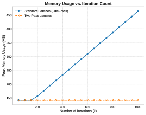
We measure the algorithm against two hypotheses on a large sparse problem with
Hypothesis 1 (Memory): The one-pass method stores the full basis
Hypothesis 2 (Runtime): The two-pass method performs
Memory Usage
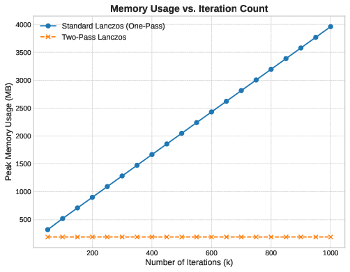
The memory data confirms Hypothesis 1 exactly. The one-pass method’s footprint scales as a straight line—each additional iteration adds one vector to the basis. The two-pass method remains flat. No allocation growth happens after initialization.
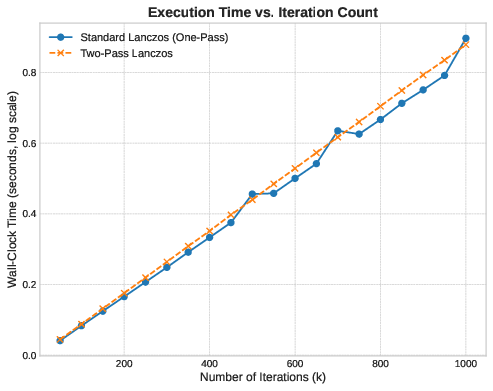
Runtime: Where Theory Breaks
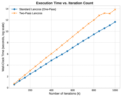
The runtime data contradicts Hypothesis 2. The two-pass method is slower, but never by a factor of two. For small
This difference comes from memory access patterns. Both methods perform matrix-vector products, but they differ in how they reconstruct the solution.
The one-pass method computes
The two-pass method reconstructs the solution incrementally. At each iteration, it operates on exactly three n-dimensional vectors:
The cost of re-computing basis vectors is less than the latency cost of scanning an
Medium-Scale Behavior
At
What About Dense Matrices?
To be sure of our hypothesis, we can test it directly using a dense matrix of size
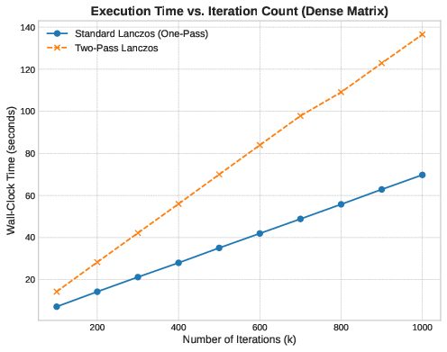
We can see that the two-pass method runs almost exactly twice as slow as the one-pass method. The slope ratio is exactly 2:1. In a compute-bound regime, the extra matrix-vector products cannot be hidden by cache effects. Here, the theoretical trade-off holds perfectly.
Scalability
Now, let’s fix the iteration count at
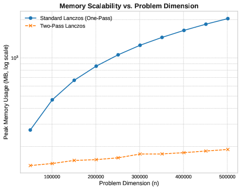
Here we have to use a logarithmic y-axis to show both curves; the two-pass line is so flat relative to the one-pass line that it’s otherwise invisible.
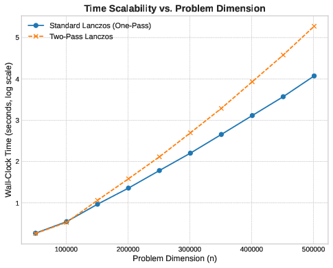
Runtime scales linearly with
As
Well, that’s it. If you want to have a better look at the code or use it, it’s all open source:
This was more of an exploration than a production-ready library, so expect rough edges. But I hope it gives an interesting perspective on how algorithm engineering and low-level implementation details can alter what seems like a straightforward trade-off on a blackboard.
Share this post on:
What's Your Reaction?
 Like
0
Like
0
 Dislike
0
Dislike
0
 Love
0
Love
0
 Funny
0
Funny
0
 Angry
0
Angry
0
 Sad
0
Sad
0
 Wow
0
Wow
0